A-B test. Is another advertising campaign more effective for an online store?

Author: Evgeny Bodyagin, https://dsprog.pro

Introduction

So, there is an online store (website). He is already running ad campaign A. There is also an alternative option: to run ad campaign B. Let’s do an A-B test to find out if the effectiveness of these campaigns is different?

Experiment Design

Null hypothesis: No performance difference between campaigns A and B.
Alternative hypothesis: There is a significant performance difference between campaigns A and B.
Processing object: Two samples of site visitor cookies mixed randomly. The sample sizes are the same.
Target Audience: Website visitors in the last 30 days.
Metrics: CTR, CR, CPC, CPA
CTR description: (number of clicks) / (number of impressions) * 100
CR description: (number of purchases) / (number of clicks) * 100
CPC description: (spend in USD) / (number of clicks) * 100
CPA description: (spend in USD) / (number of purchases) * 100
Duration of the test: 1 month
Significance levels:
α = 0.05
β = 0.2
Campaigns are launched at the same time, and the audience is divided randomly.

Leveling: Test Significance and Test Power

import scipy
# Significance level (probability of Type I error) that is used to decide whether to reject the null hypothesis.
alpha = 0.05 
# Test power (probability of type II error), which indicates the probability of not detecting a real effect if it exists.
beta = 0.2 
alpha_zscore = -1 * round(scipy.stats.norm.ppf(1 - alpha/2), 4)
beta_zscore = -1 * round(scipy.stats.norm.ppf(1 - beta), 4)
print('alpha_zscore: ', alpha_zscore)
print('beta_zscore: ', beta_zscore)

alpha_zscore: -1.96 beta_zscore: -0.8416

Determining the Minimum Sample Size

import pandas as pd
import numpy as np
import matplotlib.pyplot as plt
import seaborn as sns
from scipy import stats
sns.set()

# Initial conversion, which is taken as a starting point for comparison with other options:
baseline_cr = 0.095
# Minimum detectable effect:
min_detectable_effect = 0.005
# this content is from dsprog.pro
p2 = baseline_cr + min_detectable_effect

n = (((alpha_zscore * np.sqrt(2 * baseline_cr * (1 - baseline_cr))) + (beta_zscore * np.sqrt(baseline_cr * (1 - baseline_cr) + p2 * (1 - p2))))**2) / (abs(p2 - baseline_cr)**2)
print('Sample Size: ', round(n, 0))

Sample Size: 54363.0

Data structure

Advertising campaign (Campaign Name): The name of the advertising campaign.
Date: Date of the advertising campaign.
Impressions (of Impressions): Number of ad impressions.
Reach: Audience coverage, the number of unique users who saw the ad. Allows you to determine how many people learned about advertising.
Clicks (of Website Clicks): The number of clicks on the banner and went to the site.
Of View Content: The number of times users viewed content on the site.
of Add to Cart: The number of times users have added items to their shopping cart.
Purchases (of Purchase): The number of times users have made a purchase.
Costs (Spend /USD/): Advertising costs.
of Searches: The number of times users searched the site after clicking.

Loading data

The experiment was carried out for 1 month. Let’s load the existing data.

a_group = pd.read_csv('input/Xa_group.csv', delimiter=',')
a_group['Date'] = pd.to_datetime(a_group['Date'], format='%Y-%m-%d', dayfirst=True)
a_group.head()

	Campaign Name	Date	# of Impressions	# Reach	# of Website Clicks	# of View Content	# of Add to Cart	# of Purchase	# Spend [USD]	# of Searches
0	a campaign	2023-07-27	36908	104034	1024	2485	1028	521	2158	2609
1	a campaign	2023-07-19	129930	78269	2557	1568	1250	882	1979	1223
2	a campaign	2023-07-18	94853	110617	3126	2719	2173	922	2547	1415
3	a campaign	2023-07-30	152514	89152	3127	1955	1137	218	2454	2340
4	a campaign	2023-07-25	100917	91991	3448	2056	793	490	2356	1474

b_group = pd.read_csv('input/Xb_group.csv', delimiter=',')
b_group['Date'] = pd.to_datetime(b_group['Date'], format='%Y-%m-%d', dayfirst=True)
b_group.head()

	Campaign Name	Date	# of Impressions	# Reach	# of Website Clicks	# of View Content	# of Add to Cart	# of Purchase	# Spend [USD]	# of Searches
0	b campaign	2023-07-01	79051	47257	7431	1636	989	707	2397	2424
1	b campaign	2023-07-02	90101	63332	6070	2208	763	687	1996	1733
2	b campaign	2023-07-03	113952	52829	5376	1834	934	466	2223	2455
3	b campaign	2023-07-04	73913	105952	9453	3724	1416	218	2974	1263
4	b campaign	2023-07-05	59248	28222	8436	959	388	346	2734	1258

Calculation of metrics

a_group['CTR'] = a_group['# of Website Clicks']/a_group['# of Impressions']
a_group['CR'] = a_group['# of Purchase']/a_group['# of Website Clicks']
a_group['CPC'] = a_group['# Spend [USD]']/a_group['# of Website Clicks']
a_group['CPA'] = a_group['# Spend [USD]']/a_group['# of Purchase']

b_group['CTR'] = b_group['# of Website Clicks']/b_group['# of Impressions']
b_group['CR'] = b_group['# of Purchase']/b_group['# of Website Clicks']
b_group['CPC'] = b_group['# Spend [USD]']/b_group['# of Website Clicks']
b_group['CPA'] = b_group['# Spend [USD]']/b_group['# of Purchase']
# this content is from dsprog.pro

a_group.head()

	Campaign Name	Date	# of Impressions	# Reach	# of Website Clicks	# of View Content	# of Add to Cart	# of Purchase	# Spend [USD]	# of Searches	CTR	CR	CPC	CPA
0	a campaign	2023-07-27	36908	104034	1024	2485	1028	521	2158	2609	0.027745	0.508789	2.107422	4.142035
1	a campaign	2023-07-19	129930	78269	2557	1568	1250	882	1979	1223	0.019680	0.344935	0.773954	2.243764
2	a campaign	2023-07-18	94853	110617	3126	2719	2173	922	2547	1415	0.032956	0.294946	0.814779	2.762473
3	a campaign	2023-07-30	152514	89152	3127	1955	1137	218	2454	2340	0.020503	0.069715	0.784778	11.256881
4	a campaign	2023-07-25	100917	91991	3448	2056	793	490	2356	1474	0.034167	0.142111	0.683295	4.808163

b_group.head()

	Campaign Name	Date	# of Impressions	# Reach	# of Website Clicks	# of View Content	# of Add to Cart	# of Purchase	# Spend [USD]	# of Searches	CTR	CR	CPC	CPA
0	b campaign	2023-07-01	79051	47257	7431	1636	989	707	2397	2424	0.094003	0.095142	0.322568	3.390382
1	b campaign	2023-07-02	90101	63332	6070	2208	763	687	1996	1733	0.067369	0.113180	0.328830	2.905386
2	b campaign	2023-07-03	113952	52829	5376	1834	934	466	2223	2455	0.047178	0.086682	0.413504	4.770386
3	b campaign	2023-07-04	73913	105952	9453	3724	1416	218	2974	1263	0.127894	0.023061	0.314609	13.642202
4	b campaign	2023-07-05	59248	28222	8436	959	388	346	2734	1258	0.142385	0.041015	0.324087	7.901734

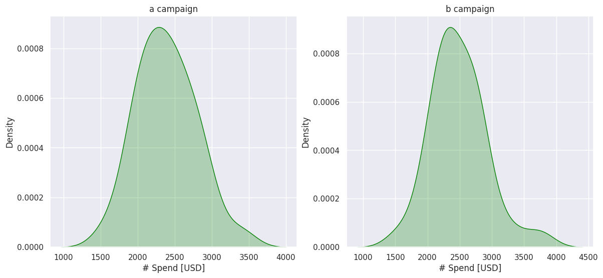
Advertising spending

fig, ax = plt.subplots(ncols=2, figsize=(14,6))

ax1 = sns.kdeplot(a_group['# Spend [USD]'], ax=ax[0], color='green', fill=True)
ax2 = sns.kdeplot(b_group['# Spend [USD]'], ax=ax[1], color='green', fill=True)
ax1.set_title('a campaign')
ax2.set_title('b campaign')

plt.show()

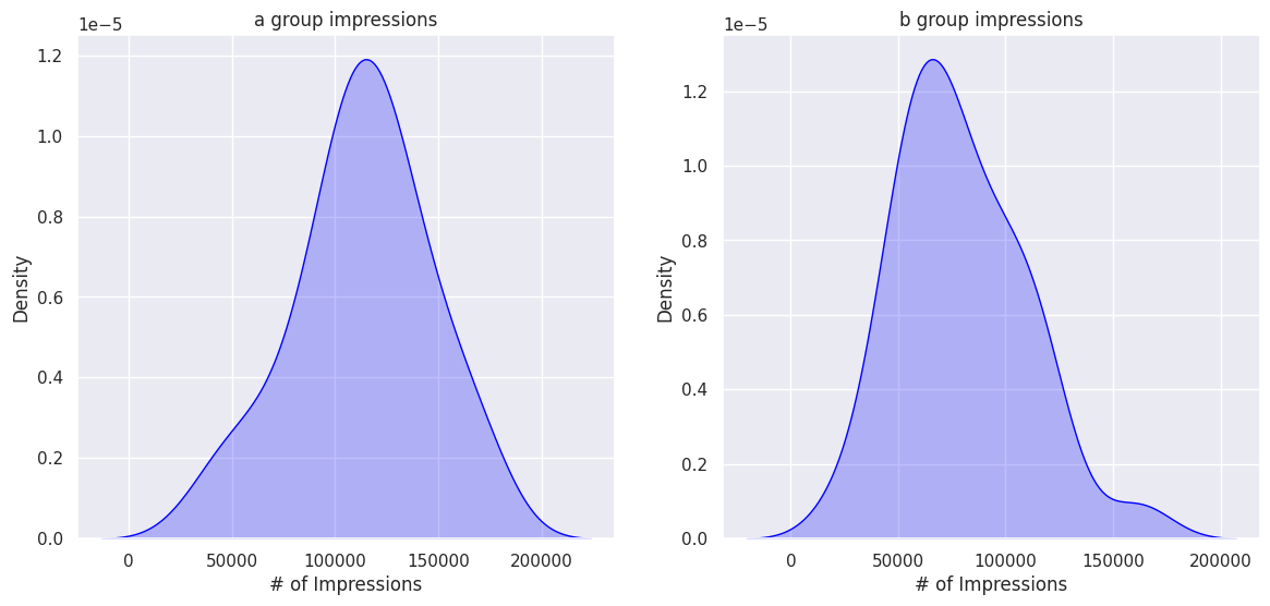
Impressions

fig, ax = plt.subplots(ncols=2, figsize=(14,6))

ax1 = sns.kdeplot(a_group['# of Impressions'], ax=ax[0], color='blue', fill=True)
ax2 = sns.kdeplot(b_group['# of Impressions'], ax=ax[1], color='blue', fill=True)
ax1.set_title('a group impressions')
ax2.set_title('b group impressions')
# this content is from dsprog.pro
plt.show()

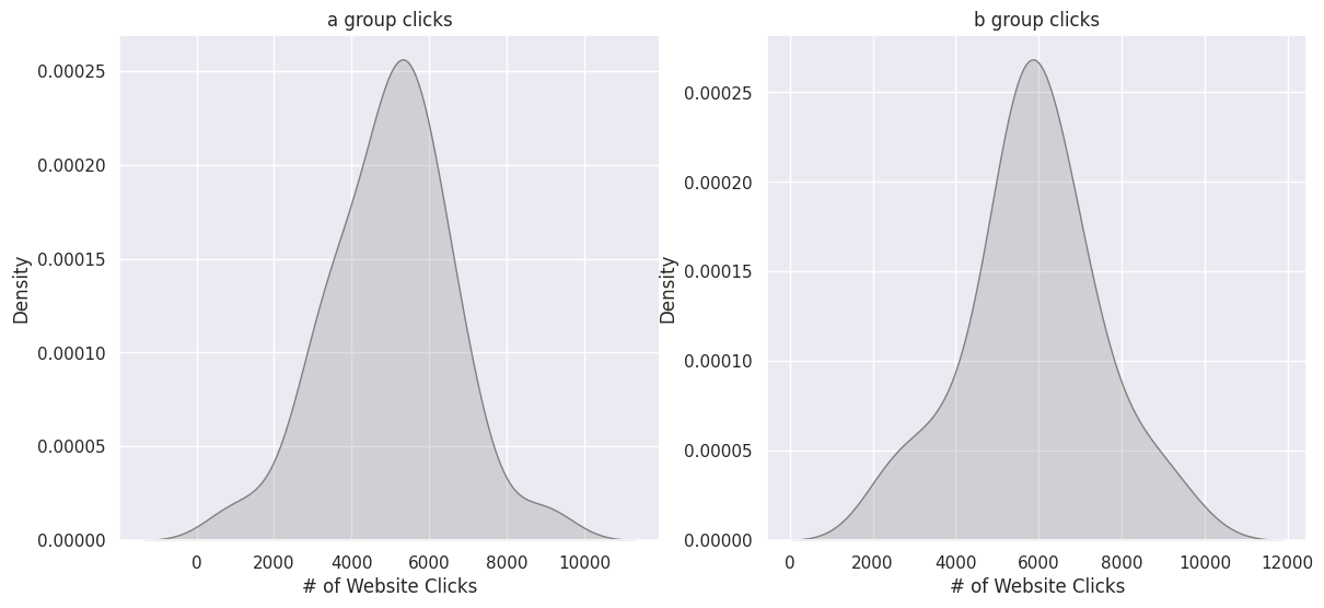
Website Clicks

fig, ax = plt.subplots(ncols=2, figsize=(14,6))
ax1 = sns.kdeplot(a_group['# of Website Clicks'], ax=ax[0], color='gray', fill=True)
ax2 = sns.kdeplot(b_group['# of Website Clicks'], ax=ax[1], color='gray', fill=True)
ax1.set_title('a group clicks')
ax2.set_title('b group clicks')
# this content is from dsprog.pro
plt.show()

Purchases

fig, ax = plt.subplots(ncols=2, figsize=(14,6))

ax1 = sns.kdeplot(a_group['# of Purchase'], ax=ax[0], color='red', fill=True)
ax2 = sns.kdeplot(b_group['# of Purchase'], ax=ax[1], color='red', fill=True)
ax1.set_title('a group purchases')
ax2.set_title('b group purchases')

plt.show()

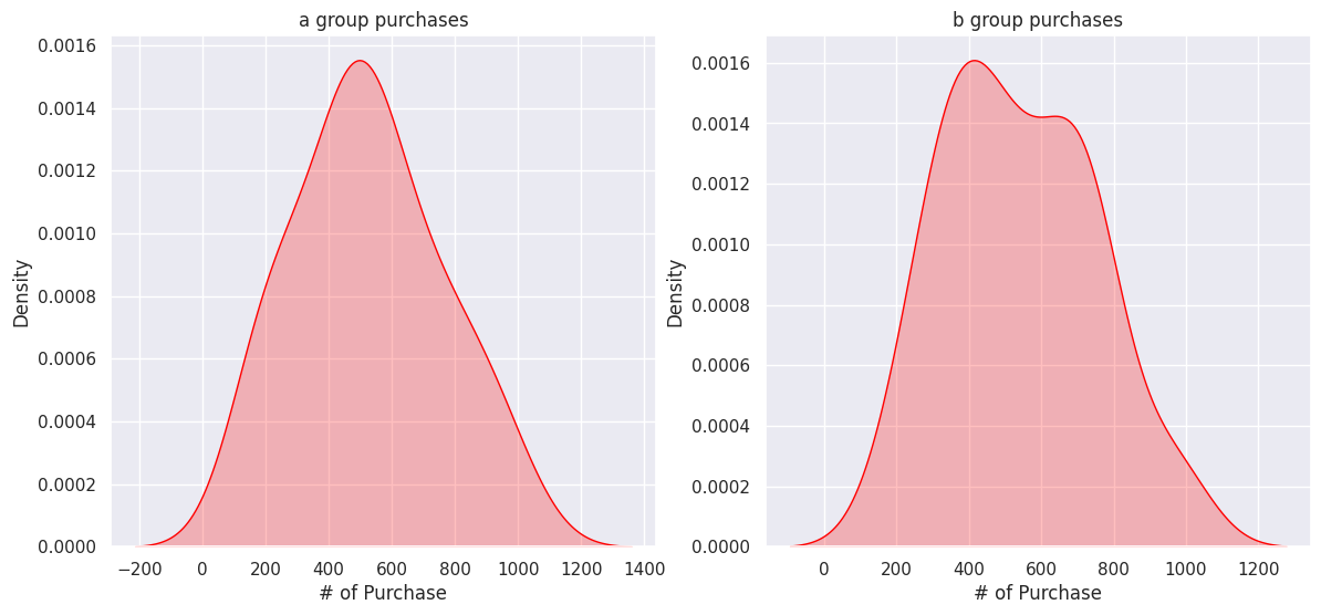
The sample sizes of A and B are comparable and appear to follow a normal distribution.

Descriptive statistics

print(a_group['# of Impressions'].describe())
print(b_group['# of Impressions'].describe())

count 30.000000
mean 113051.066667
std 32856.443638
min 36908.000000
25% 98280.750000
50% 114663.500000
75% 133569.000000
max 173904.000000
Name: # of Impressions, dtype: float64

count 30.000000
mean 79364.766667
std 29599.412623
min 24610.000000
25% 56291.500000
50% 72544.500000
75% 97436.750000
max 162153.000000
Name: # of Impressions, dtype: float64

print(a_group['# of Website Clicks'].describe())
print(b_group['# of Website Clicks'].describe())

count 30.000000
mean 4994.633333
std 1561.157185
min 1024.000000
25% 3863.750000
50% 5100.500000
75% 5734.250000
max 8928.000000
Name: # of Website Clicks, dtype: float64

count 30.000000
mean 5865.633333
std 1593.176192
min 2472.000000
25% 5275.500000
50% 5829.500000
75% 6805.250000
max 9453.000000
Name: # of Website Clicks, dtype: float64

print(a_group['# of View Content'].describe())
print(b_group['# of View Content'].describe())

count 30.000000
mean 1809.933333
std 783.556874
min 104.000000
25% 1508.750000
50% 1906.000000
75% 2204.000000
max 3361.000000
Name: # of View Content, dtype: float64

count 30.000000
mean 1873.033333
std 801.055144
min 100.000000
25% 1615.000000
50% 1816.000000
75% 2430.000000
max 3724.000000
Name: # of View Content, dtype: float64

Analysis of results

desired_palette = ["#0099cc", "#009900"]
data_all = pd.concat([a_group, b_group])
fig, ax = plt.subplots(ncols=5, figsize=(34,6))
ax1 = sns.barplot(data=data_all, x='Campaign Name', y='# of Impressions', errorbar=('ci', False), ax=ax[0], estimator='sum', palette=desired_palette)
ax2 = sns.barplot(data=data_all, x='Campaign Name', y='# of Website Clicks', errorbar=('ci', False), ax=ax[1], estimator='sum', palette=desired_palette)
ax3 = sns.barplot(data=data_all, x='Campaign Name', y='# of View Content', errorbar=('ci', False), ax=ax[2], estimator='sum', palette=desired_palette)
ax4 = sns.barplot(data=data_all, x='Campaign Name', y='# of Purchase', errorbar=('ci', False), ax=ax[3], estimator='sum', palette=desired_palette)
ax5 = sns.barplot(data=data_all, x='Campaign Name', y='# Spend [USD]', errorbar=('ci', False), ax=ax[4], estimator='sum', palette=desired_palette)

ax1.set_title('Impressions')
ax2.set_title('Clicks')
ax3.set_title('of View Content')
ax4.set_title('Purchase')
ax5.set_title('Spend [USD]')

plt.show()

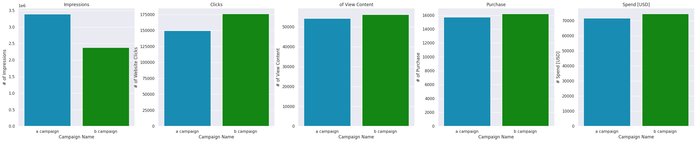
Clearly, Campaign B is more effective than Campaign A. With fewer impressions, Campaign B has more clicks and slightly more sales. It brings more user engagement in viewing the content of the site. At the same time, campaign B is slightly more expensive than campaign A.

Consider also derived indicators.

desired_palette = ["#0099cc", "#009900"]
data_all = pd.concat([a_group, b_group])
fig, ax = plt.subplots(ncols=4, figsize=(22,6))
ax1 = sns.barplot(data=data_all, x='Campaign Name', y='CTR', errorbar=('ci', False), ax=ax[0], estimator='mean', palette=desired_palette)
ax2 = sns.barplot(data=data_all, x='Campaign Name', y='CR', errorbar=('ci', False), ax=ax[1], estimator='mean', palette=desired_palette)
ax3 = sns.barplot(data=data_all, x='Campaign Name', y='CPC', errorbar=('ci', False), ax=ax[2], estimator='mean', palette=desired_palette)
ax4 = sns.barplot(data=data_all, x='Campaign Name', y='CPA', errorbar=('ci', False), ax=ax[3], estimator='mean', palette=desired_palette)
# this content is from dsprog.pro
ax1.set_title('CTR')
ax2.set_title('CR')
ax3.set_title('CPC')
ax4.set_title('CPA')

plt.show()

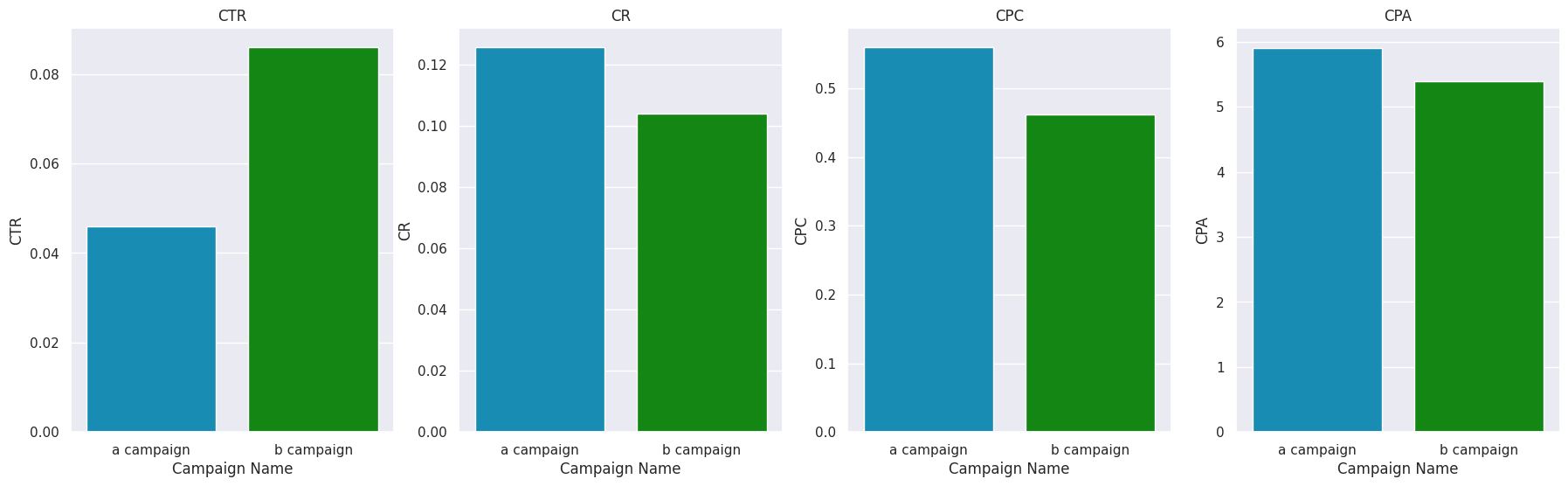
Campaign B had a much higher CTR ((clicks) / (impressions) * 100). Campaign B has a CR ((number of purchases) / (number of clicks) * 100) lower than that of campaign A. This looks a little strange. Campaign A might seem more attractive. But… notice that Campaign B has much more clicks, and Campaign B has a slightly bigger difference in sales. This explains this oddity. The CRC indicator ((costs in rubles) / (number of clicks) * 100) has the same feature as CR. The CPA ((Cost in RUB) / (Number of Purchases) * 100) indicates that Campaign B is more cost-effective.

We use statistical tests to account for differences in data; combined with significance levels (for greater confidence in the results). To do this, we will form the functions of confidence intervals:

def ratio_diff_confidence_interval(metric, measure_a, measure_b, alpha)
def cont_diff_confidence_interval(metric, alpha)

Let’s check if the difference in various metrics between the two campaigns is statistically significant.

CTR

ratio_diff_confidence_interval(metric='CTR', 
                    measure_a='# of Website Clicks', 
                    measure_b='# of Impressions', 
                    alpha=.05)

The difference in CTR between groups is 0.0297 Confidence Interval: [ 0.0293 , 0.0301 ]
Reject Null Hypothesis, statistically significant difference between a_group and b_group CTR

CR

ratio_diff_confidence_interval(metric='CR', 
                    measure_a='# of Purchase', 
                    measure_b='# of Website Clicks', 
                    alpha=.05)

The difference in CR between groups is -0.0129 Confidence Interval: [ -0.015 , -0.0109 ]
Reject Null Hypothesis, statistically significant difference between a_group and b_group CR

CPC

cont_diff_confidence_interval(metric='CPC', alpha=.05)

The difference in CPC between groups is -0.0981 Confidence Interval: [ -0.2377 , 0.0414 ]
Unable to reject Null Hypothesis, no statistically significant difference between a_group and b_group CPC

CPA

cont_diff_confidence_interval(metric='CPA', alpha=.05)

The difference in CPA between groups is -0.5102 Confidence Interval: [ -2.1616 , 1.1413 ]
Unable to reject Null Hypothesis, no statistically significant difference between a_group and b_group CPA

Conclusions

With fewer impressions, Campaign B has more clicks and slightly more sales. It brings more user engagement in viewing the content of the site. At the same time, campaign B is slightly more expensive than campaign A.

Campaign B had a much higher CTR ((clicks) / (impressions) * 100). Campaign B has a CR ((number of purchases) / (number of clicks) * 100) lower than campaign A. It looks a little strange. Campaign A might seem more attractive. But… notice that Campaign B has much more clicks, and Campaign B has a slightly bigger difference in sales. This explains this oddity. The CRC indicator ((costs in rubles) / (number of clicks) * 100) has the same feature as CR. The CPA ((Spend in USD) / (Number of Purchases) * 100) indicates that Campaign B is more cost-effective.

You can also draw the following conclusions: Based on the CTR, CR it is possible to reject the hypothesis that the effects of campaign A and campaign B are equal. The reason here is the large difference in the number:

Impressions;
clicks (of Website Clicks). Based on CPC scores, CPA cannot reject the hypothesis that the effects of Campaign A and Campaign B are equal. The reason for this is the small difference in numbers:
expenses (Spend |USD|);
Purchases (of Purchase).

As a result, we can conclude that campaign B is generally more effective than campaign A.

=======================
For the full content of this article; for cooperation with the author, write to Telegram: cryptosensors
The full content of this article includes files/data:

Jupyter Notebook file (ipynb),
dataset files (csv or xlsx),
unpublished code elements, nuances.

Distribution of materials from dsprog.pro is warmly welcome (with a link to the source).