
Author: Evgeny Bodyagin, https://dsprog.pro
Introduction
It is necessary to analyze the effectiveness of the new design for the site. We have data about site users with a conversion value for each user/session. Let’s do an A-B test. Let’s call the former design form “A”; Let’s call the new design form “B”.
Experiment Design
- Null Hypothesis: No difference in performance between Design A and Design B.
- Alternative Hypothesis: There is a significant difference in performance between Design A and Design B.
- Processing Object: Two samples of site visitor sessions mixed randomly. The sample sizes are the same.
- Target Audience: Site visitors in the last 40 days.
- Metrics: Impressions, Clicks, Purchases, Earnings
- Duration of the test: 40 days
- Levels of significance:
- α = 0.05
- β = 0.2
- Campaigns run at the same time, and the audience is divided randomly.
Data structure
- Campaign Name: The name of campaign.
- Impression: The number of ad impressions.
- Click: The number of clicks on the banner and went to the site.
- Purchase: The number of times users have made a purchase.
- Earning: Earnings after purchasing goods.
import itertools
import numpy as np
import pandas as pd
import matplotlib.pyplot as plt
import seaborn as sns
import statsmodels.stats.api as sms
from scipy.stats import ttest_1samp, shapiro, levene, ttest_ind, mannwhitneyu, pearsonr, spearmanr, kendalltau, \
    f_oneway, kruskal
# this content is from dsprog.pro
from statsmodels.stats.proportion import proportions_ztest

pd.set_option('display.max_columns', None)
pd.set_option('display.max_rows', 10)
pd.set_option('display.float_format', lambda x: '%.5f' % x)
Definition of levels: test significance and test power
import scipy
# Significance level (Probability of Type I error) that is used to decide whether to reject the null hypothesis.
alpha = 0.05
# Power of the test (probability of type II error), which indicates the probability of not detecting a real effect when it exists.
beta = 0.2
Loading data
The experiment was carried out for 40 days. Let’s load the existing data.
a_group = pd.read_csv('input/Xa_group.csv', delimiter=',')
a_group.head()
| Campaign Name | Impression | Click | Purchase | Earning | |
|---|---|---|---|---|---|
| 0 | a campaign | 77198 | 4774 | 307 | 1933 |
| 1 | a campaign | 126169 | 4285 | 574 | 2572 |
| 2 | a campaign | 114917 | 4134 | 720 | 2212 |
| 3 | a campaign | 133553 | 5144 | 545 | 1957 |
| 4 | a campaign | 90761 | 1948 | 186 | 1675 |
b_group = pd.read_csv('input/Xb_group.csv', delimiter=',')
b_group.head()
| Campaign Name | Impression | Click | Purchase | Earning | |
|---|---|---|---|---|---|
| 0 | b campaign | 115507 | 1942 | 656 | 2335 |
| 1 | b campaign | 130944 | 2844 | 606 | 2748 |
| 2 | b campaign | 175336 | 2953 | 287 | 3690 |
| 3 | b campaign | 139732 | 3550 | 709 | 2184 |
| 4 | b campaign | 108745 | 3261 | 297 | 2454 |
desired_palette = ["#0099cc", "#009900"]
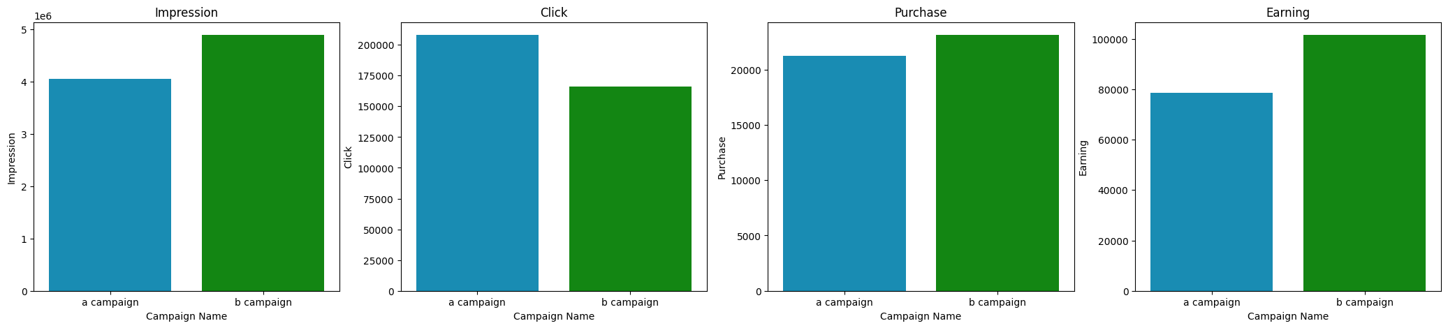
data_all = pd.concat([a_group, b_group])
fig, ax = plt.subplots(ncols=4, figsize=(26,5))
ax1 = sns.barplot(data=data_all, x='Campaign Name', y='Impression', errorbar=('ci', False), ax=ax[0], estimator='sum', palette=desired_palette)
ax2 = sns.barplot(data=data_all, x='Campaign Name', y='Click', errorbar=('ci', False), ax=ax[1], estimator='sum', palette=desired_palette)
ax4 = sns.barplot(data=data_all, x='Campaign Name', y='Purchase', errorbar=('ci', False), ax=ax[2], estimator='sum', palette=desired_palette)
ax5 = sns.barplot(data=data_all, x='Campaign Name', y='Earning', errorbar=('ci', False), ax=ax[3], estimator='sum', palette=desired_palette)
# this content is from dsprog.pro
ax1.set_title('Impression')
ax2.set_title('Click')
ax4.set_title('Purchase')
ax5.set_title('Earning')
plt.show()
Roadmap for formulating hypotheses
- Assumption that the data is normally distributed (normality)
- Assumption that the dispersion is homogeneous (homogeneity).
Both assumptions will be tested through a test of statistical significance. The type of tests will be selected for each task. If both assumptions are valid, then two independent sample t-tests are applied. If one of the assumptions can be rejected, the Mann-Whitney U-test (non-parametric test) will be applied.
Note: The t-test is used to test for the existence of a statistically significant difference between the two group A and group B by looking at the means. This is a parametric test.
Shapiro-Wilk test
There are many tests for normality. The most famous of them are the criterion:
- Chi-square test;
- Kolmogorov-Smirnov criterion;
- Lilliefors criterion;
- Shapiro-Wilk normality criterion. Let’s use the last one.
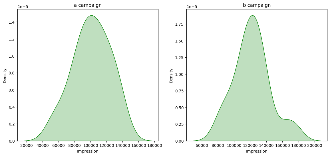
Unable to reject Null Hypothesis for “Impression” in “group A”, because “Test Stat group A” = 0.9810 and “p-value_a” = 0.7250 Unable to reject Null Hypothesis for “Impression” in “group B”, because “Test Stat group B” = 0.9609 and “p-value_b” = 0.1801
Unable to reject Null Hypothesis for “Click” in “group A”, because “Test Stat group A” = 0.9882 and “p-value_a” = 0.9465 Unable to reject Null Hypothesis for “Click” in “group B”, because “Test Stat group B” = 0.9709 and “p-value_b” = 0.3851

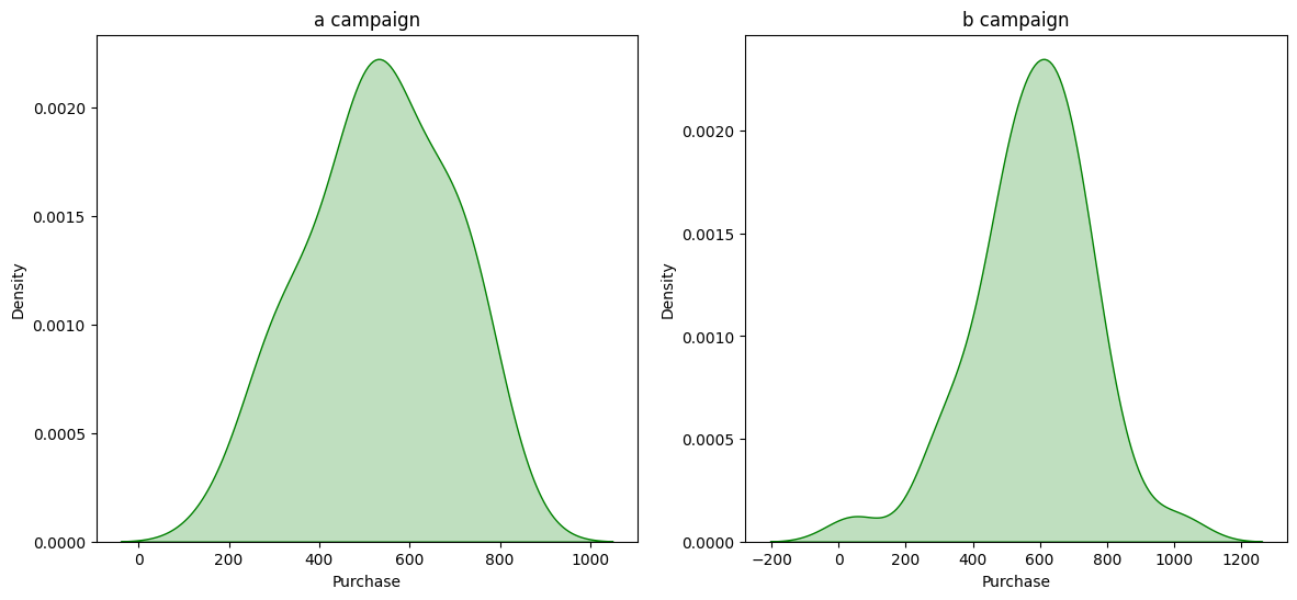
Unable to reject Null Hypothesis for “Purchase” in “group A”, because “Test Stat group A” = 0.9775 and “p-value_a” = 0.5972
Unable to reject Null Hypothesis for “Purchase” in “group B”, because “Test Stat group B” = 0.9690 and “p-value_b” = 0.3341
Unable to reject Null Hypothesis for “Earning” in “group A”, because “Test Stat group A” = 0.9790 and “p-value_a” = 0.6524 Unable to reject Null Hypothesis for “Earning” in “group B”, because “Test Stat group B” = 0.9734 and “p-value_b” = 0.4570

So. None of the indicators: Impression, Click, Purchase cannot reject the null hypothesis about the normality of the distribution.
Levene test
We run Levene’s test to see if there are significant differences in variation between groups.
columns = ["Impression", "Click", "Purchase", "Earning"]
for column in columns:
    test_stat, pvalue = levene(a_group[column], b_group[column])
    if (pvalue < alpha):
        print('Reject Null Hypothesis for "%s" because "Test Stat" = %.4f and "p-value" = %.4f ' % (column, test_stat, pvalue))
    else:
        print('Unable to reject Null Hypothesis for for "%s" because "Test Stat" = %.4f and "p-value" = %.4f ' % (column, test_stat, pvalue))
Unable to reject Null Hypothesis for for “Impression” because “Test Stat” = 0.5893 and “p-value” = 0.4450
Unable to reject Null Hypothesis for for “Click” because “Test Stat” = 0.0978 and “p-value” = 0.7553
Unable to reject Null Hypothesis for for “Purchase” because “Test Stat” = 0.0232 and “p-value” = 0.8793
Unable to reject Null Hypothesis for for “Earning” because “Test Stat” = 0.2993 and “p-value” = 0.5859
So. None of the indicators: Impression, Click, Purchase can not reject the null hypothesis of the absence of significant differences in the variations between groups.
According to the hypothesis formulation roadmap defined above, this means that we can apply two independent sample T-tests.
T test
columns = ["Impression", "Click", "Purchase", "Earning"]
for column in columns:
    test_stat, pvalue = ttest_ind(a_group[column], b_group[column], equal_var=True)
    if (pvalue < alpha):
        # this content is from dsprog.pro
        print('Reject Null Hypothesis for "%s" because "Test Stat" = %.4f and "p-value" = %.4f ' % (column, test_stat, pvalue))
    else:
        print('Unable to reject Null Hypothesis for for "%s" because "Test Stat" = %.4f and "p-value" = %.4f ' % (column, test_stat, pvalue))
Reject Null Hypothesis for “Impression” because “Test Stat” = -4.1173 and “p-value” = 0.0001
Reject Null Hypothesis for “Click” because “Test Stat” = 2.7901 and “p-value” = 0.0066
Unable to reject Null Hypothesis for for “Purchase” because “Test Stat” = -1.2474 and “p-value” = 0.2160
Reject Null Hypothesis for “Earning” because “Test Stat” = -7.0324 and “p-value” = 0.0000
So, using the t-test, we determined the only parameter (Purchase) that does not have a statistically significant difference between group A and group B. For the rest of the parameters, it is possible to reject the null hypothesis.
Subtotal
Considering that all indicators have a normal distribution, as well as the absence of significant differences in the variations between groups, it is possible to complete the data processing.
The conclusion is this. The new design B has an impact on performance:
- Impression,
- click,
- Earning
The new design B has no effect on the score:
- Purchase
However, it is possible to create a combined function that, taking into account normality, the significance of variations, used or did not use the Mann-Whitney U-test (non-parametric test).
Mann-Whitney U-test in data processing
columns = ["Impression", "Click", "Purchase", "Earning"]
for column in columns:
    hypothesis_checker(a_group, b_group, column)
========== Impression ==========
*Normalization Check:
Shapiro Test for Control Group, Stat = 0.9810, p-value = 0.7250
Shapiro Test for Test Group, Stat = 0.9609, p-value = 0.1801
*Variance Check:
Levene Test Stat = 0.5893, p-value = 0.4450
Independent Samples T Test Stat = -4.1173, p-value = 0.0001
H0 hypothesis REJECTED, Independent Samples T Test
========== Click ==========
*Normalization Check:
Shapiro Test for Control Group, Stat = 0.9882, p-value = 0.9465
Shapiro Test for Test Group, Stat = 0.9709, p-value = 0.3851
*Variance Check:
Levene Test Stat = 0.0978, p-value = 0.7553
Independent Samples T Test Stat = 2.7901, p-value = 0.0066
H0 hypothesis REJECTED, Independent Samples T Test
========== Purchase ==========
*Normalization Check:
Shapiro Test for Control Group, Stat = 0.9775, p-value = 0.5972
Shapiro Test for Test Group, Stat = 0.9690, p-value = 0.3341
*Variance Check:
Levene Test Stat = 0.0232, p-value = 0.8793
Independent Samples T Test Stat = -1.2474, p-value = 0.2160
H0 hypothesis NOT REJECTED, Independent Samples T Test
========== Earning ==========
*Normalization Check:
Shapiro Test for Control Group, Stat = 0.9790, p-value = 0.6524
Shapiro Test for Test Group, Stat = 0.9734, p-value = 0.4570
*Variance Check:
Levene Test Stat = 0.2993, p-value = 0.5859
Independent Samples T Test Stat = -7.0324, p-value = 0.0000
H0 hypothesis REJECTED, Independent Samples T Test
The results of the combined function are no different from the previously announced intermediate conclusions. However, it has the potential to calculate cases where a non-parametric criterion is needed.
Conclusions
Both design options A and B are characterized by “Impression”, “Click”, “Purchase”, “Earning”. None of the indicators: Impression, Click, Purchase cannot reject the null hypothesis about the normality of the distribution. None of the indicators: Impression, Click, Purchase can not reject the null hypothesis of the absence of significant differences in the variations between groups. These two facts made it possible to apply the parametric T-test. As a result of this test, it was found that only one parameter (Purchase) did not have a statistically significant difference between group A and group B. Thus, there is a significant difference in efficiency between design options A and B.
Additionally, a combined function was created which, taking into account the normality, significance of variations, either uses or does not use the Mann-Whitney U-test (non-parametric test). It has the potential to calculate cases where a non-parametric criterion is needed.
=======================
For the full content of this article; for cooperation with the author, write to Telegram: cryptosensors
The full content of this article includes files/data:
- Jupyter Notebook file (ipynb),
- dataset files (csv or xlsx),
- unpublished code elements, nuances.
Distribution of materials from dsprog.pro is warmly welcome (with a link to the source).