Author: Evgeny Bodyagin, https://dsprog.pro

Introduction

You need to test the effectiveness of the new web application design. There is the old design “A”, there is a new design “B”. Let’s do an A-B test. Let’s make a reservation that there are many variations of conducting A-B tests. It is necessary to take into account the nuances of the analyzed object/process in each individual case. This material will show the basic steps of the A-B test.

Experiment Design

• Null Hypothesis: No difference in performance between Design A and Design B.
• Alternative Hypothesis: There is a significant difference in performance between Design A and Design B.
• Processing Object: Two samples of site visitor sessions mixed randomly. The sample sizes are the same.
• Target Audience: Site visitors in the last 30 days
• Metrics:
• Duration of the test: 30 days
• Levels of significance:
• α = 0.05
• Campaigns run at the same time, and the audience is divided randomly.

Data structure

Each row of data represents information about user visits to web applications.

• User ID (User_ID): User ID.
• Campaign_Name): Campaign name (design A or design B).
• View content (View): The number of times the user has viewed content on the site.
• Clicks: Number of clicks per banner. The number of users who used design A and design B are equal.

import pandas as pd
import numpy as np
import matplotlib.pyplot as plt
import seaborn as sns
%matplotlib inline
import sys

import warnings
warnings.filterwarnings('ignore')
from scipy.stats import mannwhitneyu

alpha = 0.05 

Loading data

alldata = pd.read_csv('input/Xab_group.csv')
df_userAgg = pd.read_csv('input/Xab_group.csv')
alldata.head()

	User_ID	Campaign_Name	View	Click
0	1	a campaign	4.0	0.0
1	2	b campaign	12.0	0.0
2	3	a campaign	1.0	0.0
3	4	a campaign	5.0	0.0
4	5	a campaign	8.0	0.0

Check for duplicates and null values

alldata.duplicated().sum()

0

alldata.isnull().sum()

User_ID 0
Campaign_Name 0
View 0
Click 0
dtype: int64

There are no duplicate values in the original data; there are no null values either.

grouped = alldata.groupby('Campaign_Name')
a_group = grouped.get_group('a campaign')
b_group = grouped.get_group('b campaign')

desired_palette = ["#0099cc", "#009900"]
data_all = pd.concat([a_group, b_group])
fig, ax = plt.subplots(ncols=2, figsize=(18,6))
ax1 = sns.barplot(data=data_all, x='Campaign_Name', y='View', errorbar=('ci', False), ax=ax[0], estimator='sum', palette=desired_palette)
ax2 = sns.barplot(data=data_all, x='Campaign_Name', y='Click', errorbar=('ci', False), ax=ax[1], estimator='sum', palette=desired_palette)
# this content is from dsprog.pro
ax1.set_title('View')
ax2.set_title('Click')

plt.show()

a_group_View_sum = a_group['View'].sum()
b_group_View_sum = b_group['View'].sum()
a_group_Click_sum = a_group['Click'].sum()
b_group_Click_sum = b_group['Click'].sum()

print('A group View sum: %s'%(a_group_View_sum))
print('B group View sum: %s'%(b_group_View_sum))
print('A group Click sum: %s'%(a_group_Click_sum))
print('B group Click sum: %s'%(b_group_Click_sum))

A group View sum: 149422.0
B group View sum: 151117.0
A group Click sum: 10423.0
B group Click sum: 12133.0

Design B is more efficient than design A. Both indicators show a positive effect. But… do our findings have statistical significance?

A-B test

Calculate the averages for each indicator; for each group: A and B. We also calculate the differences in the average values.

columns = ['View', 'Click']
obs_diffs = {}
for column in columns:
    view_cont= alldata.loc[alldata['Campaign_Name']=='a campaign'][column].mean()
    view_test= alldata.loc[alldata['Campaign_Name']=='b campaign'][column].mean()
    print('Mean of %s "a campaign": %s\n' % (column, round(view_cont,3)))
    print('Mean of %s "b campaign": %s\n' % (column, round(view_test,3)))
    
    obs_dif_vw= view_test - view_cont
    obs_diffs[column] = obs_dif_vw
# this content is from dsprog.pro
    print('Diff means of %s : %s\n' % (column, round(obs_dif_vw,3)))
    print("**************")

Mean of View “a campaign”: 4.981
Mean of View “b campaign”: 5.037
Diff means of View : 0.056

Mean of Click “a campaign”: 0.347
Mean of Click “b campaign”: 0.404
Diff means of Click : 0.057

Let’s apply the bootstrap technique to estimate the difference in the mean values of variability between the groups a campaign and b campaign by repeatedly generating random samples and calculating the difference in the means. Let’s form histograms based on the results.

columns = ['View', 'Click']
boxes_data = {}

for column in columns:
    n_iterations = 10000
    group_control = alldata[alldata['Campaign_Name'] == 'a campaign'][column].values
    group_test = alldata[alldata['Campaign_Name'] == 'b campaign'][column].values
    
    
    diffs_viw = np.empty(n_iterations)
    np.random.seed(200)
    # this content is from dsprog.pro
    for i in range(n_iterations):
        random_indices = np.random.choice(len(group_control), len(group_control), replace=True)
        sample_control = group_control[random_indices]
        sample_test = group_test[random_indices]
        
        diffs_viw[i] = np.mean(sample_test) - np.mean(sample_control)
        
    diffs_view = np.array(diffs_viw)
    boxes_data[column] = diffs_view
    low, high = np.percentile(diffs_view, 2.5), np.percentile(diffs_view, 97.5)
    
    plt.figure(figsize=(6,5))
    plt.xlabel(column + ': proportions of differences', fontsize=15)
    plt.ylabel(column + ': frequency', fontsize=15)
    plt.axvline(x= low, color= 'r', linewidth= 2)
    plt.axvline(x= high, color= 'r', linewidth= 2)
    plt.hist(diffs_view)

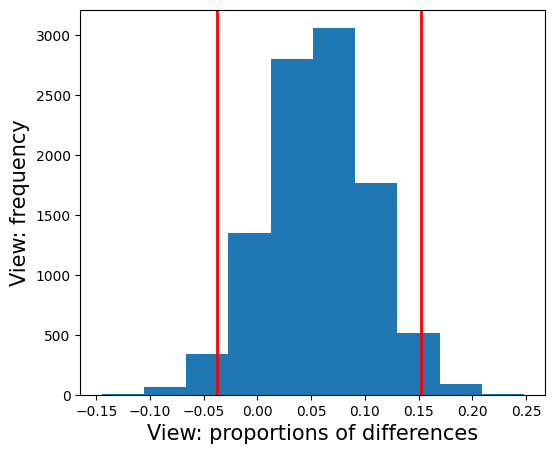
For each indicator, we will make a comparison between the p-value and the alpha level to accept or refute the null hypothesis.

The p-value for View is: 0.1218
Unable to reject Null Hypothesis, no statistically difference between “a group” and “b group” 0.1218 > α on View

The p-value for Click is: 0.0
Reject Null Hypothesis, statistically significant difference between “a group” and “b group” 0.0 < α on Click

Conclusions

By the View indicator, we cannot reject the 𝐻0 hypothesis. The new form of design did not bring statistically significant changes to the rate of page views by users of the web application. However, the new design had a statistically significant impact on the click rate. Thus, in general, there is still a significant difference in performance between design A and design B.

======================
For the full content of this article; for cooperation with the author, write to Telegram: cryptosensors
The full content of this article includes files/data:

• Jupyter Notebook file (ipynb),
• dataset files (csv or xlsx),
• unpublished code elements, nuances.

Distribution of materials from dsprog.pro is warmly welcome (with a link to the source).